Automated Market Makers (AMMs) have become an integral part of the DeFi ecosystem, facilitating trillions in trading volume. Pioneered by projects like Bancor and Uniswap in 2017/2018, AMMs provide an interesting alternative to the traditional central limit order book model.
Replicating an order book on the blockchain runs into two major problems: first, there are gas costs involved for each order a maker wants to submit or change, which becomes expensive over time and inefficient. Second, since blockchain data is publicly available and readily accessible, frontrunning prevents traders from executing the trades they actually want.
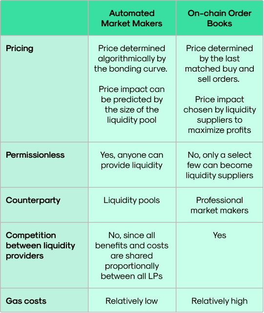
One of the major advantages of AMMs over order books is that anyone can supply assets to a pool to become a liquidity provider and earn trading fees. As a result, AMMs are able to attract more capital, resulting in greater market depth for decentralized exchanges (DEXes) as compared to their centralized counterparts. It’s no surprise then that this innovation has become a major foundation for the most popular DEXes and even other DeFi applications.
A Brief History of AMMs
Operating a DEX on the blockchain with AMMs was first discussed by Ethereum co-founder Vitalik Buterin back in 2016, which later inspired the creation of Uniswap.
While Bancor is credited with creating the first ever AMM (called omnipool), a major disadvantage of this approach was that tokens had to be paired against the protocol’s native BNT token. Since this token was used as a common denominator across all pools, all swaps required the BNT token. As a result, traders experienced slippage twice if they wanted to swap from USDC to ETH (since the overall route is: from USDC to BNT, then from BNT to ETH).
By getting rid of the need for a network token to make swaps as in Bancor, trades on Uniswap fully depend on the token reserves in a liquidity pool, thanks to a simple but elegant formula: x * y = k (more on that in the next section) that revolutionized DeFi. The success of Uniswap since its launch in November 2018 eventually spawned the creation of dozens of similar AMM-based DEXes and proved that AMMs held a lot of promise as a new financial primitive.
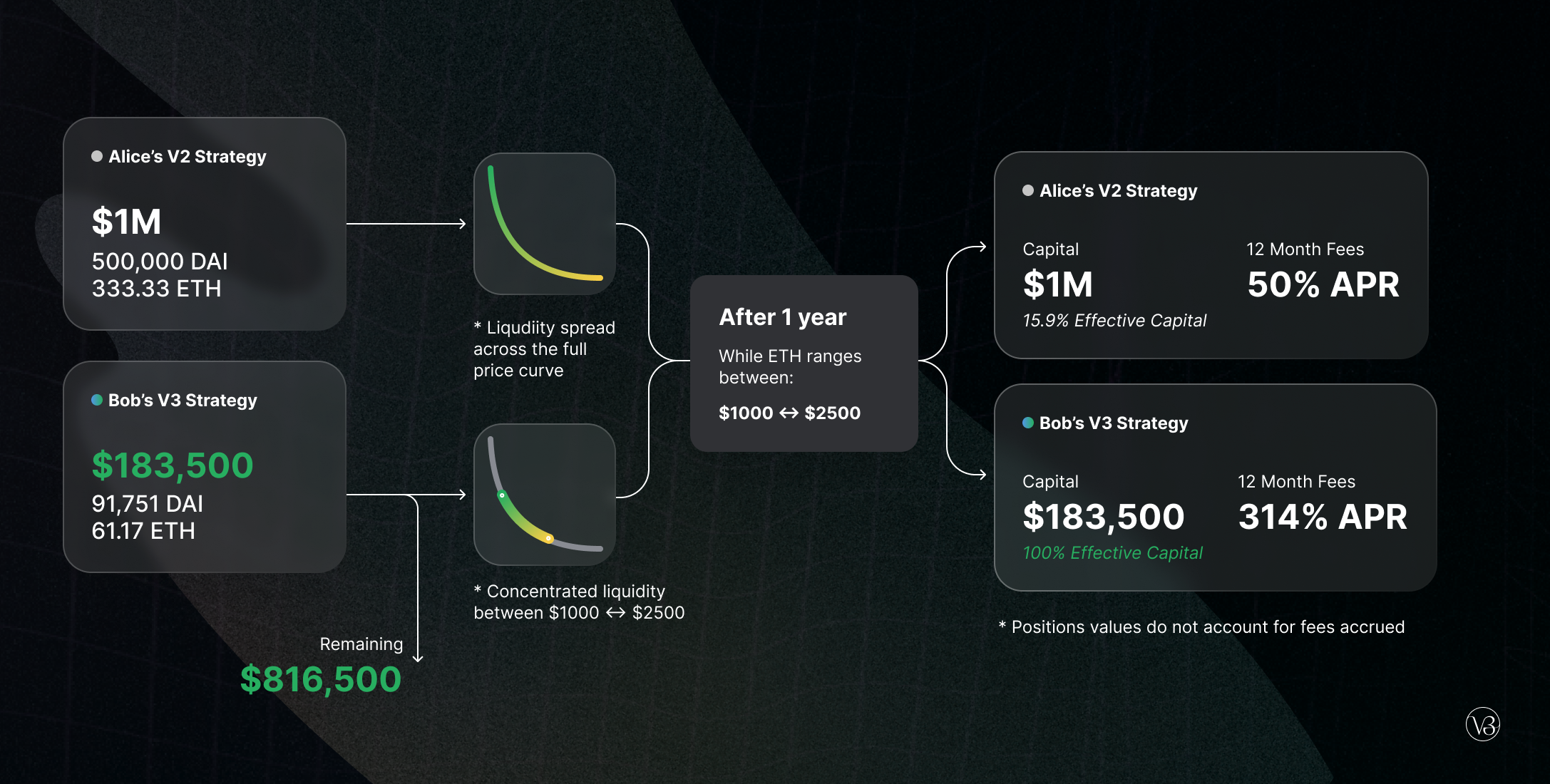
While Uniswap made great strides with its first two implementations, given that liquidity is provided evenly across the entire price range from zero to infinity, capital efficiency was lacking. This problem was solved with the introduction of concentrated liquidity in Uniswap v3, where capital efficiency was vastly improved, which resulted in greater liquidity and lower slippage.
For LPs, it reduces the risk of impermanent loss due to liquidity being provided in a price range. Another favorable aspect of concentrated liquidity is the simplicity and flexibility it enables, with Uniswap v3 being able to assume the form of any possible AMM.
For more on the history behind AMMs, check out this detailed post.
Now we know a bit about the background of AMMs, let’s look at how they function.
AMMs Explained
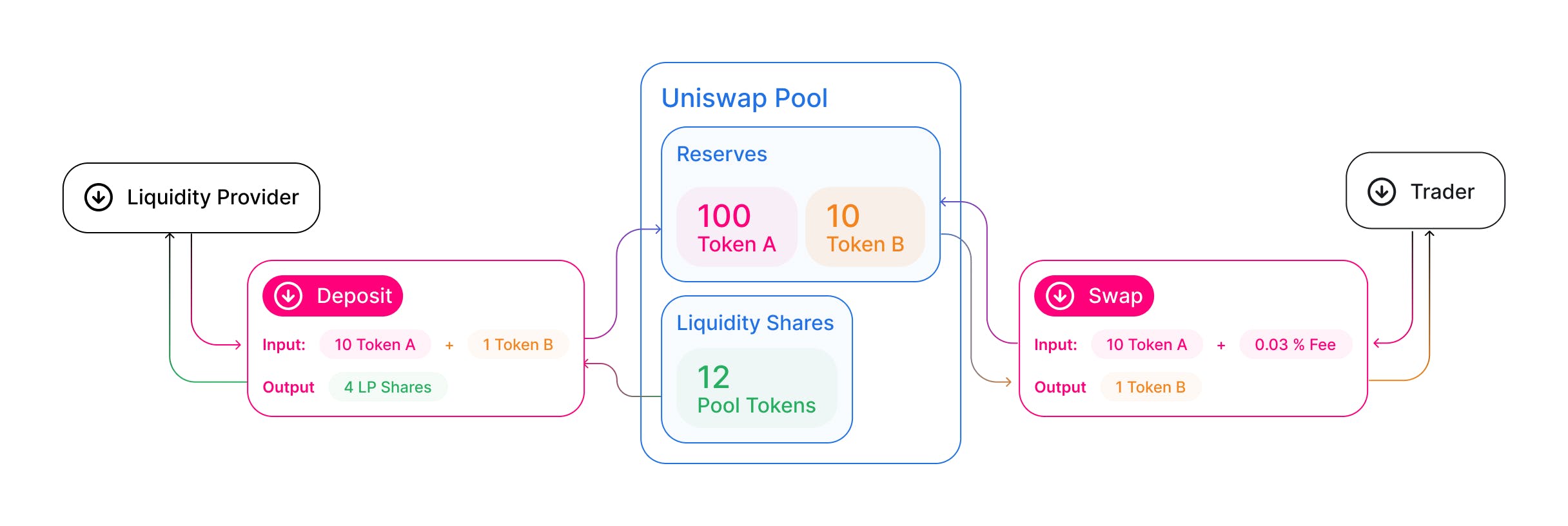
To facilitate trading, AMMs replace order books with liquidity pools. A liquidity pool is basically a smart contract that holds reserves of two different tokens in a particular proportion. The smart contract’s code specifies how prices are determined by the reserves, the rules for liquidity provision and trading, as well as the fees incurred by traders when swapping via the pool.
Liquidity providers (LPs in the following) can supply crypto-assets to a pool’s reserve to earn trading fees from each transaction and receive token rewards for supplying liquidity to a particular pool. Token rewards are usually issued in the protocol’s governance token, which gives holders voting rights on the development of the protocol and its AMM.
To track the share of fees an LP will receive, pool shares are credited as LP tokens in proportion to their liquidity contribution as a fraction of the entire pool. That means if an LP supplies 10% of the assets, they’ll earn 10% of the trading fees generated by the pool. The LP tokens which represent their liquidity position can be burned at any time to remove liquidity from the pool.
The major innovation of AMMs over the order book model is that anyone can provide liquidity and earn a share of the trading fees, lowering the barriers to participation. In the centralized order book model, the role of an LP is usually reserved for a select few high net worth individuals or companies. With the advent of AMMs, this role is opened up to a much wider audience.
From a trader’s perspective, the advantage is that they can obtain liquidity immediately by interacting with a pool, and there’s no need to wait for a matching order. If a trader wants to buy or sell a token, they can go to the pool, specify the asset and the amount they want to trade. The smart contract will then provide an exchange rate based on the bonding curve, which is calculated according to the reserves of the two different tokens in the pool.
As an example, consider a pool for ETH-USDC with the following reserves: ETH = 1,500,000 and USDC = 10,000. Following the Uniswap v2 model, the AMM price equals the ratio of the reserves (150 USDC). Once the trader buys 1 ETH with $150 in USDC, the AMM removes 1 ETH from the pool and credits these tokens to the trader’s wallet. The AMM also adds the trader’s 150 USDC to the pool. Depending on the fee parameter, which is set and calculated by the smart contract, the trader will be charged a percentage of their transaction.
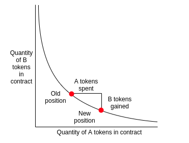
Source: https://ethresear.ch
After the trade has been executed, there’ll be slightly less ETH in the pool and slightly more USDC. Since the bonding curve algorithmically determines the price of ETH as the ratio between the asset quantities, the price of ETH falls to around 147 USDC. If the trader had sold ETH for USDC instead, then the ratio would have moved in the opposite direction and caused the price of ETH to increase.
For larger trade sizes, the difference between the spot price and realized price (also known as slippage) becomes larger as the amount of tokens traded relative to the size of the pool increases. Therefore, AMMs force those entering larger trades to pay a higher price as compared to smaller trades. Therefore, some slippage tolerance must be set for orders to be executed.
When a trade occurs that causes the price quoted by the pool to diverge significantly from the wider market value, then arbitrageurs can step in and readjust the pool quantities to profit from the difference in prices on the AMM and other trading venues.
For example, if a large sale of ETH caused the price to crash from 150 USDC to 135 USDC, but the market average remains close to 150 USDC, then arbitrageurs can buy ETH from the AMM and proceed to sell it on other trading venues. As more ETH is bought through the AMM by arbitrageurs and more ETH is removed from the liquidity pool, the price will eventually converge with the market price of 150 USDC.
As we’ve seen above, any swap alters the asset composition of the pool and the exchange rate is automatically updated, changing the value of the entire pool. As an asset’s price fluctuates, so does the pool value, meaning that the value of the LP’s pool share also oscillates. Ideally, an LP wants to remove liquidity as close as possible to the price they entered the position, since they may realize a loss when assets are taken out of the pool after a price change, known as impermanent loss. However, impermanent loss may be outweighed by the fees and token reward earned by the LP.
AMMs in Action
In this section, we’ll examine three popular AMM models to highlight the different approaches: Uniswap, Curve, and Balancer.
Uniswap
There are different variations of AMMs with varying bonding curve designs.
The Constant Product Market Maker model regulates the price by keeping the mathematical product of the amounts of two assets constant. For example, Uniswap versions 1 and 2 are known as CPMMs where the multiple of the amount of two different tokens is kept constant according to the following formula:
x * y = k
Where x is the quantity of one token (e.g., ETH), y is the quantity of another token (e.g., USDC) and k is a constant.
In v2, the pool’s smart contract assumes that the reserves of the two assets have equal value. So an LP would have to provide ETH and USDC in a 50:50 ratio to the pool to maintain the constant k.
Source: Uniswap Docs
In v3, liquidity provision can be concentrated on a portion of the bonding curve, reducing the slippage and improving capital efficiency. LPs in v2 would provide liquidity across the entire price range of the bonding curve, which means a lot of the liquidity doesn’t get consumed. With concentrated liquidity, the LPs can pick a range in which they would provide liquidity and can adjust their positions based on market conditions.
Source: Uniswap blog post
Therefore, Uniswap v3 moves away from the constant product model, blending this model with a constant sum market maker. Trades do not take place along the single level curve determined by the x * y = k equation, as in previous versions. Liquidity can be discontinuous, meaning that each LP’s position could be drained of a single reserve, which cannot happen with v1/v2.
*Learn more about how Uniswap v3’s AMM functions in the whitepaper. *
Curve
Curve is an example of a hybrid function market maker, combining the constant product and constant-sum models to provide an automated market maker that is more efficient for stablecoin swaps.
A Curve v1 liquidity pool consists of two or more assets with the same peg, such as USDC and DAI, WBTC and renBTC, or stETH and ETH. As stablecoins have experienced a massive uptick in adoption, Curve has become the DEX with the largest total value locked, facilitating stable swaps with very low fees and slippage.
As the assets in a pool become imbalanced, the bonding curve takes the form of a constant-product curve (similar to Uniswap v1/v2). However, when the assets are supplied in such a way that the exchange rate is close enough to parity, then the bonding curve shifts to a constant sum model:
x + y = k
The benefit of a constant sum approach is that it eliminates slippage found in the constant product models. The hybrid model used by Curve is illustrated by the ‘Stableswap invariant’ in the figure below:
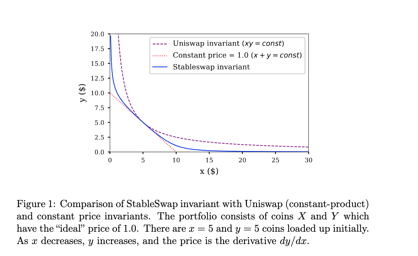
Source: https://curve.fi/files/stableswap-paper.pdf
To dive deeper into the mechanism underlying Curve v1, check out the StableSwap whitepaper.
In Curve v2, the price scale is constantly updated according to an internal price oracle to better represent the market price and ensure trading remains near the equilibrium point. The market maker function can be pegged to any price, which suits all tokens instead of stablecoins or assets that trade in tandem.
Balancer
The Balancer protocol allows each pool to have more than two assets and to be supplied in any ratio. Each asset reserve is given a weight at pool creation where the sum of weights is equal to 1, where the weights do not change with the provision or removal of liquidity, instead representing the value of the reserve as a fraction of the pool’s value.
Balancer generalizes the constant product concept applied by Uniswap to a geometric mean, giving rise to what is termed a Constant Mean Market Maker. This model also adds another player in the AMM aside from LPs and traders, known as controllers, who are tasked with managing a pool.
x^(0.2) + y^(0.3) + z^(0.5) = k
With Balancer’s smart pools using a constant mean formula (such as the one shown above), we can create liquidity pools with up to eight tokens, permitting more customizability.
Therefore, Balancer’s pools are like index funds that construct a portfolio of assets with fixed weights. The graphic below compares the curve used by Balancer with two assets (one weighted 25% and the other 75%) compared to the Uniswap v2 curve.
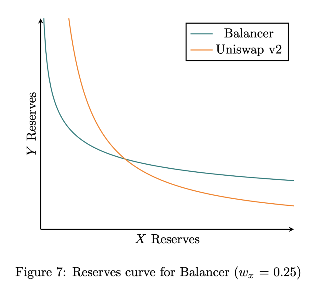
Source: Paradigm
For example, we can specify any weight for a bullish or bearish pool. A bullish pool for ETH-USDC can be created by specifying a weight of 90% for ETH and 10% for USDC. Alternatively, a bearish pool can be launched by doing the opposite.
Read Balancer’s whitepaper for more details on their AMM implementation.
Other DeFi Applications of AMMs
DEXes are just one use case of protocols using the AMM algorithm, which also forms the basis for other applications in DeFi.
One notable example is Balancer’s Liquidity Bootstrapping Pools (LBPs). LBPs are used for fair token launches, with Perpetual Protocol being the first project to do so with the $PERP token. Unlike the AMMs we have explored so far, the parameters of the pool can be changed. A two-token pool is set up with the project token, such as PERP, and a collateral token, such as USDC.
It initially set the weights in favor of the project token, then gradually flip to favor the collateral token by the end of the sale. Token sales can be calibrated so that the price declines to the desired minimum. In this way, an AMM is utilized to function similarly to an auction, where early buyers will pay a higher price, and over time, the project token’s price declines until the allocation is completed.
We can find good examples of applications of AMMs in DeFi outside of DEXes in automated lending, with projects such as Notional Finance and Yield Protocol. Both projects facilitate fixed-rate, fixed-term crypto-asset lending and borrowing with a constant power sum bonding curve.
The AMMs in these cases are designed for trading of ERC-20 tokens similar to zero-coupon bonds that are redeemable for the underlying asset at a particular future date. A constant power sum curve incorporates time to maturity into the pricing, permitting users to trade based on interest rates rather than price.
AMMs are one of the defining innovations emerging from the DeFi space and have led to the creation of a variety of decentralized applications, including DEXes and automated lending. Research into different and enhanced variations is still ongoing (such as TWAMM) that further expands the design space and the emergence of a new generation of protocols built using AMMs.
Further Reading
-
Automated Market Makers and Decentralized Exchanges: a DeFi Primer
-
A Mathematical View of Automated Market Maker Algorithms and Its Future
-
SoK: Decentralized Exchanges with Automated Market Maker Protocols